Introduction

I’ve been listening to Prefuse 73 and Pogo lately, who are electronic music producers defined by their aggressive use of track sampling in order to create melody and harmony, rather than taking the more “direct” approach of sampling individual instruments. This creates for very stylistic music where you can almost hear the individual brush strokes of sound - this song a great example of this.

I’ve also been looking at some cool projects that perform image/video reconstruction built off of simpler shapes, using a genetic algorithm.

For example, this project can reconstruct an image from shapes or text! Like, perhaps, a grayscale Mona Lisa reconstructed with letters of the alphabet:

Well, an image is just a two dimensional signal, and audio is just a one dimensional signal, so why couldn’t I, instead of visually approximating an image, “audially” approximate some music, just like Prefuse 73? (but probably far worse)

A (very) brief primer on genetic algorithms

Genetic algorithms, at least the kind I’m thinking of, are actually very simple in theory!

Firstly, you need an input target signal and a set of “building block” signals (we’ll call these the individuals of a population). You can really transform and combine the individuals together in however way you want in order to get a set of “descendant” individuals - offspring, if you like. Then, you score every individual, seeing how well they fit your end goal. The worst fitting individuals are removed, and the remaining individuals are, again, transformed in various random ways to get some more descendants. This process repeats a few more times, after which we take the very best individual we found, add it to our output signal, and the start the entire process over again.

We keep doing this until we’re happy with how closely we’ve managed to approximate our end goal.

This is called a genetic algorithm because it’s a lot like how genetic evolution works. Offspring of a population are slightly different to their ancestors, and this can either make them a better or worse fit for the environment. The best offspring go on to survive and proliferate further, and the worst offspring die off.

Audio and musical audio

Now to tackle this problem more concretely, we need to figure out some key details. We know audio is represented as a series of scalar samples (the sampling rate is not very important as long as it’s consistent). Since it is a signal, there are a lot (read: infinite) different transformations we could apply, but, let’s not forget we are working with music. With that in mind, how could we transform the signal without losing it’s “musicality”?

We could…

• Split the signal
• Reverse the signal
• Change the pitch/speed
• Change the amplitude
• Add two signals together (crossover)
• Apply low/high shelf gain

There are definitely also some other ways we could transform music samples that I missed, but I’d like to keep it simple for now. We will randomly select and use these transformations with random parameters to create our sample descendants (our “offspring”).

Again, in keeping with simple transformations, the signal will just be split randomly at some point in the middle 2/4ths, producing the left and right slice. I’m also not going to employ any special techniques for adjusting pitch and speed independently, I’m just going to resample it to a frequency ratio based on a random number of cents, changing both speed and pitch simultaneously.

I’d like to use a large sample library of entire songs, but sampling entire songs seems… suboptimal. It would be a good idea (purely guided by intuition) to pre-slice the sample library into smaller chunks of, say, 5 seconds to work with.

Perhaps the biggest difference to image reconstruction is that we can’t change the color content of our samples like we can with visual media. When picking a point on the image to place a new sample, you can take an average color of that area and use that value to recolor the sample, essentially giving some “hints” to the genetic algorithm.

For audio, we could actually do something even more powerful and pick the best offset for a sample based on its similarity using an operation called cross-correlation. For the unaware, cross-correlation is an operation on two signals which is best described as sliding one signal across another, and for each offset we create a new signal of their dot product (the dot product can be used as a measure of signal similarity). If we do this for our sample, the maxima of the cross-correlation signal gives us not only the best offset where similarity of the signals is highest, but also a value which we can use to measure the fitness of the sample.

A worked example

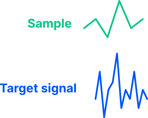
So to sum up my ideas: We start with a target signal, and set of sample signals. In our example, let’s just use a single sample signal (generation 0):

We can transform that sample signal in various ways to create descendants (generation 1):

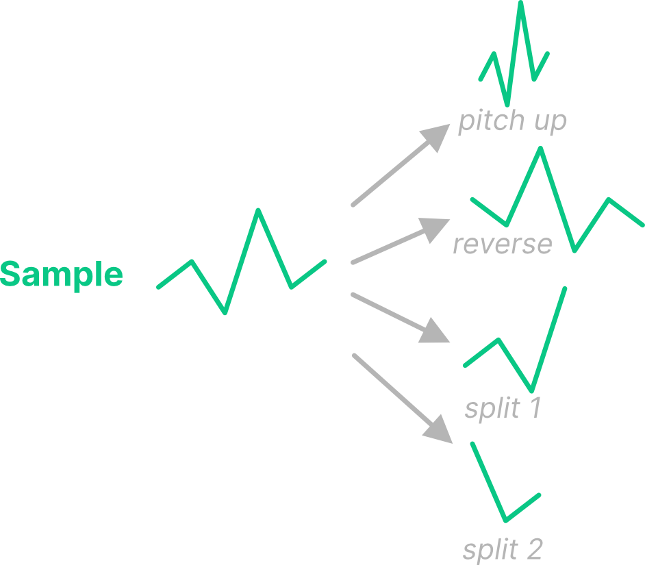
Let’s just look at one of these descendants now - the reversed sample. We can run another generation of transformations. For example, the reversed sample could be pitched up (generation 2).

After we’ve gone through a few generations, we should now have quite a few variations of that initial sample we started with. We’ll run cross-correlation for each one and look at the peak value. Let’s see what happens with that reversed and pitched up sample in generation 2:

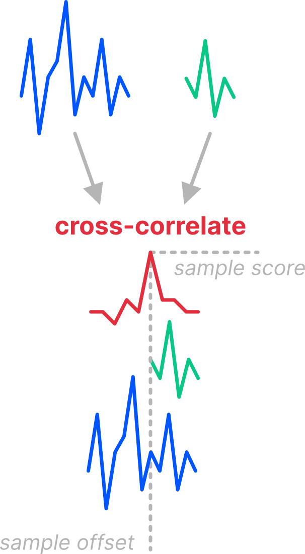
We see a peak in the cross-correlation signal, telling us two things: 1. Where the sample fits best in the signal (on the x-axis), and 2. The similarity at that place where it fits best (on the y-axis).

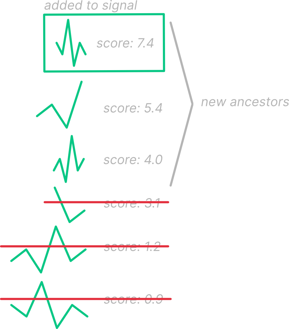
Now we can order all the transformed samples from every generation by their similarity score (based on the peak value), and take the very best sample to add to our output signal. We can also use the top percentile of signals as generation 0 for the next generation and drop the worst ones.

At a snail’s pace

After throwing together some code (in Rust, of course) and fixing up some small bugs, it was… slow. Very. Very. Slow. With approximately 2000 5-second samples, even after reducing all the parameters, it couldn’t get past a single generation on my 6-core AMD CPU within an hour (after which point I just stopped it).

To be completely honest, I sort of gave up on this project for a few days as I really didn’t have any ideas to significantly speed it up. I knew I would definitely need some 100-1,000 (or maybe even 10,000) generations to get any decent result out, but that would take, quite literally, weeks to compute. The cross-correlation step was just far too expensive.

I eventually got an idea which, on paper, made a lot of sense (and to be honest I don’t know why I didn’t think of it earlier). The idea was to “seed” the offspring with the results of the ancestor’s cross-correlation peak delay. This meant that we only had to do a cross-correlation with the entire target signal once (on the very first generation). Every subsequent cross-correlation could conservatively only look at the signal within the same approximate vicinity as the seed. This is based on the idea that if an ancestor best fit at a given delay X, it’s most probable that the descendants would also best fit at a given delay X, plus or minus some epsilon. This, of course, meant that cross-correlation would be much faster as we could significantly narrow down our search space. However to prevent things from getting too comfortable in one position (genetic algorithms are really about shaking things up as much as possible whilst also converging on a solution), we’ll ignore the seeding every, say, 10 generations - I’ll call these “seed reset generations”.

Indeed, this worked excellently and each generation after the initial “seeding” generation was roughly 8-10x faster.

Stuck in the middle of nowhere

I was excited to hear what it could produce now that I could actually run 100 or so generations! What came out was quite underwhelming. The output signal was mostly silence, occasionally broken by a few samples. I was expecting to hear roughly 1000 samples (outputting 10 of the best samples per generation). It seemed like the same of the few samples were being placed in the same spot, essentially overwriting what was already there in the previous generation. This is a well-known phenomenon in genetic algorithms and is called premature convergence.

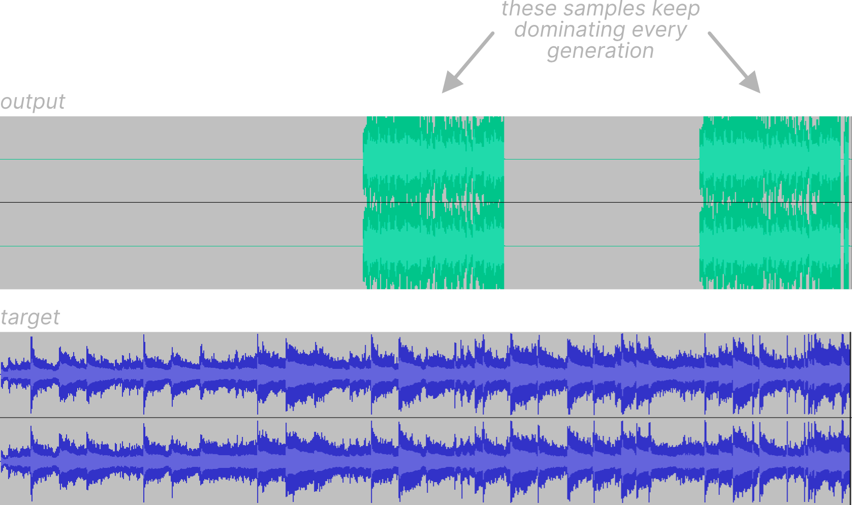
Now, I did hazard a guess that the reason this was happening was because I had implemented elitism. Elitism is an optional step in a genetic algorithm where some top percentile of the current generation directly survives into the next generation. Unfortunately, what can happen here is that those elite candidates continue to dominate on subsequent generations and the rest of the population doesn’t have a chance to be selected. This is problematic because there definitely are other candidates that have potential to become a very good solution (after a few generations), but are only suppressed. In other words, our solution is stuck in the middle of nowhere.

After doing some light research on this issue (lucky me, genetic algorithms are quite well-researched), there seemed to be two options:

• Cross your fingers and mutate more aggressively: The internet people told me this fit better for a small search space
• Apply elitism more strategically

The first approach did indeed make sense for a small search space, but I highly doubted it would work well for my situation as randomly stumbling upon a really good solution from a batch of bad solutions would be exceedingly unlikely and thus would take an unreasonable number of generations (keep in mind, at 44.1 kHz and 60 seconds of audio, that’s over 2.6 million “genes” - my search space is very large).

So what’s the second approach all about? Well, having a simple fixed elitism percentile would quickly cause premature convergence, so how else could we apply elitism? I saw a couple ways:

• Begin to apply elitism towards the end of the algorithm, with little to no elitism at the start where initial solutions are being figured out
• Use the fitness score as random weighting to pick the elite

I eventually decided on doing a combination of the two, wherein we do very little elitism at the start, and when we do carry out elitism, we do so by randomly selecting samples by means of a linear probability density over the sorted population. Instead of directly using the fitness scores as probability values, a linear (read: triangular) distribution function blind to the actual scores should give the weaker samples an even better chance at being selected.

Onwards to the optima

Up until this point, I didn’t have much information about what the algorithm was doing as it ran. Most of my changes were guided by educated guesses after looking at the output. The issue still remained where samples ended up dominating a specific region and nothing else was being done, so after outputting some simple logs for each generation and assigning IDs to each initial sample, I noticed that elitism, even at a small amount, had a drastic effect on genetic diversity. Even after elitism was only just being introduced, at maybe 1-2 elites per generation, a single genetic “archetype” would begin dominating and ruin the results. As I was only running 50-100 generations, I figured that elitism would only become benefitial at much later generations, perhaps some 1000 generations down the line. As such, I disabled elitism while I tried to figure things out.

In another attempt to shake things up and force more diversity, I implemented “false seeding”. This reuses the same seeding logic as before, but instead we pick a random, false/misleading seed as a new possible transformation of samples, so that samples can be forced to explore other possible delays without the cost of a seed reset generation. This definitely helped a little, so I figured I was on the right track to giving my algorithm more momentum to escape the valley of local optima.

Yet another idea that I had completely missed before was to work on the target signal in sections. For example, instead of running 100 generations over the entire target signal, we run 100 generations over the first 10 seconds of the target signal, the next the 10 seconds, and so on. Then only at the end do we stitch together each section’s output. This should prevent the “tunnel vision” effect we saw before.

The new output was looking much healthier than before and definitely had more variation, but it still seemed to be focusing in on only one part of each section a little too often. I tried to squeeze more granularity out of it by reducing the sample chunking to 1 second, and the target chunking to 5 seconds. This helped to even out the distribution of sample delays somewhat, but I figured it was time to tackle this problem head-on.

The first solution I tried was to track the regions of output audio that hadn’t been touched yet and give a little boost to the score of samples which would fill those untouched areas. This helped out a little, but really not as much as I had anticipated. I’m still not sure exactly why this is, but I estimate that the score scaling wasn’t strong enough to overcome the top competitors.

Looking at the log output once more, it was clear that many of the samples were being placed very close to each other (obviously). In order to prevent this, I implemented a simple mechanism which, in each generation, checked that the samples being added to the output weren’t too close in proximity to other samples that have already been added in that generation - this helped enormously and now the output signal started to flesh out and become coherent.

Tearing it down

I had made good progress thus far and thought all that was left to do was run it for more generations with a richer sample set. However, as I was perusing through some similar projects, it critically dawned on me that cross-correlation probably wasn’t as appropriate as I had thought. There was another metric likely better suited that I really wanted to explore: Peak signal-to-noise ratio. I feared this would produce much better results than cross-correlation, because I felt if it did, it would render a lot of my work so far as a waste of time.

For the unaware, peak signal-to-noise ratio (PSNR) is a fairly simple metric for quantifying how well one signal reconstructs another. Mathematically, it’s the average of the squared distance between two signals (also known as the mean squared error (MSE)), as a ratio (dB) of the maximum value. It’s mostly used to measure image/video compression fidelity - but there’s no reason we can’t generalize it to audio too. Actually, since we only care about comparing fitness scores, we don’t need to normalize the MSE to get the PSNR, we can just use the MSE directly. There’s only one downside with this new fitness metric: We can’t find the best fitting delay for each sample, the delay will just have to become another random parameter. On the other hand, scoring samples should be much faster as there is no FFT involved! So all in all, the computation time should balance out as each generation should be faster, but we’ll just need far more of them. This does mean, however, that I’d be scrapping the seeding logic, proximity filtering, and a heap of other things I had done so far.

Waveforms tell me everything and nothing

Even after fiddling with using MSE as a fitness function, I was feeling defeated. The scoring just, quite plainly, sucked. The output was disappointing, and I didn’t really know what to do. This moment was really just a testament to “do your research first”, because after looking at papers that did a similar thing with sound synthesis, I realized that waveforms didn’t give me enough information. Sound is complex but the way it’s represented as waveforms is deceptively simple. A one-dimensional series of samples cannot by itself show us the actual information we want - that is, mainly, the frequency content. The frequency content of sound is quite important in music as the relationships between those frequencies make up intervals, and stacked intervals make up chords, and intervals also make up melody. Analysing how the air pressure wobbles around tells me exactly nothing about that!

So how do we address this? We move our signal into a different space! Namely, we transform our audio into a spectrogram, and use the spectrograms for our scoring. Spectrograms are fascinatingly powerful; they don’t require any additional data to construct, yet can reveal so much about the signal (they can even be used to identify speech!).

To really demonstrate what I mean, here’s the spectrogram of that same target signal as before:

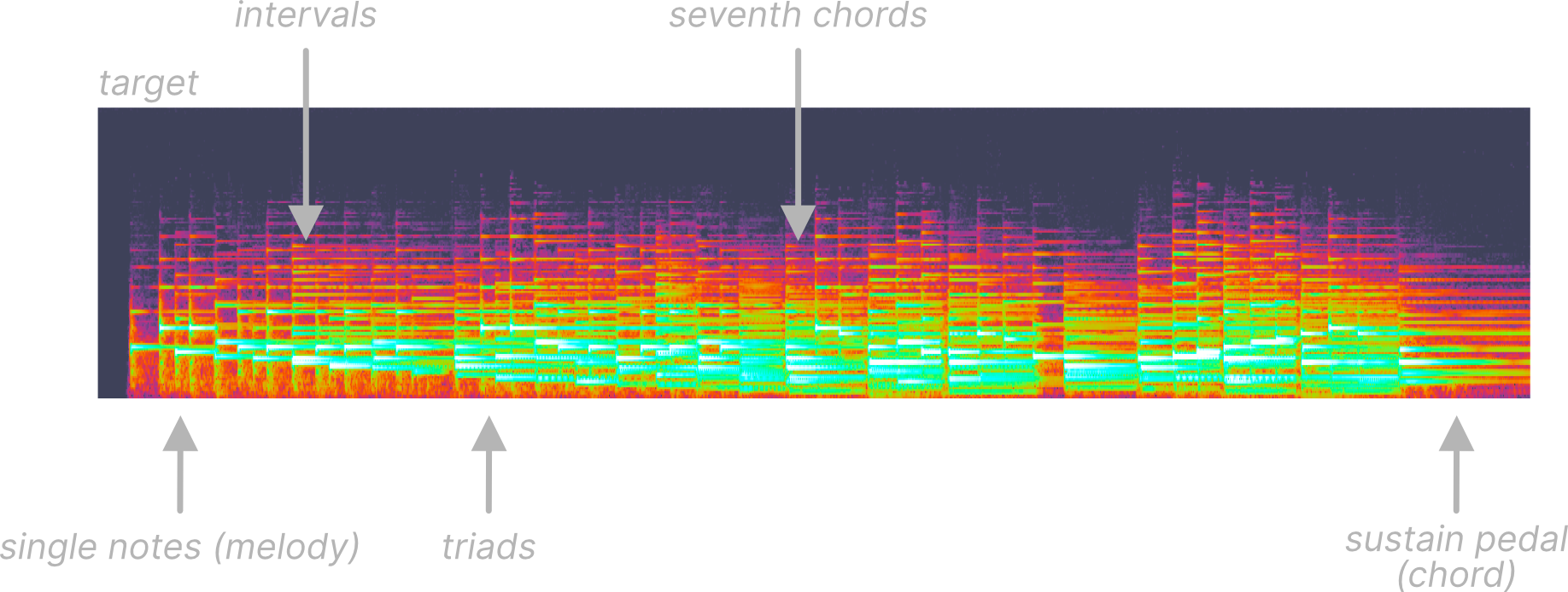
The key here is that now our fitness function can be “aware” of these concepts in the sound, instead of blindly trying to compare the waveforms. We should just be able to reuse the existing MSE function (which this paper calls the “Spectral Norm”), but instead over the spectrogram values.

After putting together an implementation of this heuristic, I found that any need for the “hacks” I previously used dissolved away. The system had great variety out the box thanks to this new spectrogram-based scoring, placing diverse samples (with diverse transforms) across a broad range of delays, filling out the space. I did need to filter out samples that were too quiet (with an RMS threshold), and opted to add a “restart generation” wherein the population is reset every N generations to the initial starting population to bounce out of local optima.

In fact, I was feeling so confident in the performance of the genetic algorithm that I felt now would be the right time to pull away all the remaining guiderails: I removed all the sample chunking and preprocessing and pretty much gave the algorithm as much freedom as I could give. I ran it on various target songs with some different sample sets and the output at the earlier generations was quite acceptable, however as it went on, the population tended towards shorter and shorter sample durations, stabilizing at around 0.2-0.3 seconds per sample. I’m sure that’s just where the fitness function led it, but I figured I needed to give it some “artistic direction”, as having many tiny samples didn’t really fit the style of music I was going for. More generally, what I thought would be best was to, instead of giving the genetic algorithm hard guides to follow, nudge it in different artistic directions by way of scaling scores based on various (completely subjective) parameters.

Strictly increasing cycles

One thing that I didn’t consider in depth was how randomising the delay instead of determinstically selecting it off the cross-correlation affected the efficacy of the genetic algorithm as a whole. Each generation we have a set of individuals, all with a score based on a completely (psuedo)random delay, which we then rank by and select the top to be written to the output. The issue is then when the next generation comes by, those “best” parents were only the “best” at those specific delays they were randomly chosen for: If the delay was anything else, it’s score could’ve been much lower - as such, there’s absolutely no guarantee that the offspring of the best parents will even score well. So then, for this particular model, we really need to consider the children side-by-side with the parents. Those children will also have their own uniquely random delay, but it could very well score better than the parent because of that.

This is where I introduce a concept I decided to name cycles. There’s probably an actual name for it, but that’s what I’m calling it. Essentially, each cycle, we run N generations. I’ll get to how N is “calculated” later, but for each cycle we run N mutation passes and N sorting/elimination passes, but we never specifically discard the parents! The parents may very well be discarded if they score too low, but then again, so could the children. In this model, the children and parents are ranked alongside each other, almost as if they’re from the same generation. This should, in theory, be more appropriate for my specific application, and should open up opportunities for “late-bloomer” samples to get a chance. Another huge benefit of this design is that local optima are much less frequent since for each cycle, the population is reset back to the starting population.

Great, but how is N calculated? Running a fixed number of generations per cycle I found isn’t actually all that optimal and plateaus quickly. The most obvious solution here is to simply keep track of the best score we saw in the last cycle, and only if the best score in the current cycle exceeds that previous score, then we can stop and move onto the next cycle. This ensures the population never regresses in fitness and the final output is strictly improving. As I anticipated, this turns out to be N=1 for the first few 20 cycles where progress is being made easily, then begins to climb up to N=2 then N=3 (and so on) generations per cycle as the output gets better and better.

It was finally at this point in the project where I began to feel satisfied with what it was producing and only needed to polish some things up. The only final major change I had to make was to lazily evaluate the waveforms of mutations on-demand instead of processing them on-the-spot, in order to avoid the OOM that occurred when I bumped up the sampling rate to 48 KHz. This makes some transformations run distributively on the offspring, e.g., a pitched-up sample that has been split will have each split be pitched-up individually, but if anything, this should give the genetic algorithm even more freedom.

The results

You may have noticed I haven’t included any audio samples up until this point. That’s half because most of it is either completely incomprehensible garbage or complete silence (as per some silly bugs), but half because I thought it would be fun to put together an album of what it created (cherrypicked, of course). For the album I employed some special techniques in order to actually use my software. In no particular order:

• Use the target song itself as a sample library
• Swapping the sample library out between cycles
• Swapping the target song out between cycles
• Restricting possible transformations
• Permitting score regression between cycles
• Injecting a false initial output signal

An unintentional feature is that I could do almost all those things by simply copying WAV files around. As such, I consider the filesystem the main user interface for my program, which is very nice.

As for the genres of music, I went with my favourite jazz standards as target music, and the sample library was… all over the place. To be honest, there was no strategy to choosing samples, I just picked what I thought would sound cool (a lot of it ended up being D&B/Jungle). Many tracks on the album don’t actually sound anything like the target music - this really comes down to two things: 1. Approximating jazz (trumpets, swung acoustic drums, piano, acoustic bass) with D&B (electronic instruments, synths, spliced up drum breaks) is about as tricky as it sounds, and 2. I never wanted to have a perfect copy of the melody and harmony anyway.

The project itself is open-source under MIT on my GitHub - it’s only a couple files of Rust code, one of which is just a set of utility functions for audio. All the parameters you can tweak are right at the top with comments explaining what they do. I tried to make the algorithm as readable and concise as possible so feel free to play with it.

Conclusion

Overall this project ended getting way further than I anticipated, but there are still a lot of ideas here that I left unexplored. For instance, in retrospect, it would’ve been possible to reuse the cross-correlation logic but on the spectrogram in two dimensions; at the cost of making the fitness function even more expensive. As for the output itself… it’s okay (for a computer). Quite obviously it doesn’t have the same creative touch as a human and lacks any cohesiveness, but I would say it’s mildly tolerable to listen to. I would guess it doesn’t work as well as similar projects that use genetic algorithms on images because because an image has all it’s details observable at a single moment in time. With music, all the details are stretched out across a few minutes and it’s far more difficult to get away with approximations in that way. That’s just my speculation, anyway.

The entire post unintentionally turned into a big development diary from planning to completion of this little experiment, but I hope there was at least one thing that was useful or interesting!